Localization

To make a car follow a trajectory, we first need to know where the car is. There are two levels: local localization (relative to the surroundings) and global localization (relative to a shared coordinate frame / map). The global one is needed for path planning and to exploit map information (signs, lane markings). This post surveys the localization approaches — GPS, visual localization, road-map localization — then codes one visual-localization example (PnP + RANSAC) on Argoverse, connecting directly to the BA built in the SLAM post.

VO gives relative motion; SLAM builds a map and localizes simultaneously. Localization is the last piece: using a map (or GPS, a road map, an HD map) to find the global pose of the car — and it must run real-time, since every downstream driving decision needs the position right away.

Contents

• Satellite positioning (GPS/GNSS)
• Visual localization: 4 directions
• Example: feature-based localization with PnP on Argoverse
• Road-map localization
• Putting it together: VO – SLAM – Localization
• Real-world deployment: sensor fusion
• Trends 2025–2026

Satellite positioning (GPS/GNSS)

The idea: we know the satellite positions, measure the distance to them (via signal travel time), then intersect spheres to find our position — typically needing 4 satellites (3 for position, 1 to cancel the receiver clock bias).

Two important concepts:

• GDOP (Geometric Dilution of Precision): with noisy distances, where the satellites sit in the sky matters as much as how many there are. Each measured distance is a band of uncertainty (not a thin sphere), and your position lies where these bands intersect. Satellites spread wide (large intersection angle) ⇒ a small, compact intersection ⇒ good localization; satellites clustered in one direction ⇒ a narrow angle ⇒ an elongated smear ⇒ large uncertainty. GDOP packs this whole geometric effect into a single number.
• DGPS (Differential GPS): a ground station at a precisely known location measures its own GPS error (since it knows the truth), then broadcasts that correction so nearby receivers can subtract the same atmospheric error — pushing accuracy from a few metres down to a few centimetres (the advanced version is RTK-GNSS).

Limitations of GPS:

• Availability — signal lost in tunnels, urban canyons (tall buildings block it).
• Accuracy — a few metres (raw GPS) → a few cm (DGPS/RTK + IMU).
• Position only — no heading (rotation) unless fused with an IMU.
• Low rate — 5–10 Hz (≈ 0.1–0.2 s per fix) while vehicle control needs ~100–1000 Hz.
• Multipath — in built-up areas the signal reflects off walls, corrupting the timing; the position can jump by hundreds of metres.

→ GPS alone is not enough. This is why we need visual localization and sensor fusion.

Visual localization: 4 directions

The common idea: pre-build a map/database of known places with their features (usually 3D landmarks, each carrying a descriptor of its appearance, extracted from images or laser during mapping — e.g. with SLAM). At localization time: take features from the current image/scan and look them up in the database to infer the pose. The four main directions:

1. Topometric — instead of computing a precise pose, it asks: “which stored frame does my current view look most like?”. The whole image is summarized into a single global vector; we find the nearest vector in the database and return its frame ID (inferring the pose where that frame was taken) — not a full 6DoF pose. The map is a directed graph whose nodes are frames (a node is added only after the car has moved past a distance threshold, so a stationary car doesn’t create redundant nodes). A discrete Bayes filter tracks the location over time, so accuracy improves as you go.

2. Deep learning — a CNN directly predicts the 6DoF pose (3D position + 3D rotation) from one RGB image. Pro: less thrown off by wrong matches (outliers) than feature-based methods. Con: less accurate, the pose is only an approximation of the ground truth.

3. Feature-based — connects directly to BA. The map consists of 3D points, each with a descriptor (SIFT/SURF/deep). For a query image: extract descriptors → match against the database via fast approximate search (kd-tree, inverted index, FLANN…) instead of brute force. This is the example we will code.

4. Map-based — no pre-built feature map needed, only a free road map (OpenStreetMap) + relative motion from VO.

Example: feature-based localization with PnP on Argoverse

Feature-based is the direction that connects directly to the BA in the SLAM post. The core difference:

In BA we optimize the camera poses and the 3D points jointly. In localization the 3D points are fixed (already in the map) — we only solve for the pose. The problem is much smaller and has a closed-form solution: that is PnP (Perspective-n-Point), finding (R, t) that minimizes the reprojection error of the known 3D points projected into the image.

To picture it: it’s like walking into a familiar room — you recognize a few objects (the 3D points known from the map), and just from how they look from where you stand (their 2D positions in the image) you work out where you are and which way you’re facing. That is exactly what PnP does.

Another difference: because the map is huge and we use approximate search, a lot of matches are wrong (>50%, sometimes >80%). So geometric verification with RANSAC is mandatory:

• Take a minimal set of 3 correspondences (each point gives 2 observations $x, y$ ⇒ $3\times2 = 6$ = the number of pose parameters) to solve the pose extremely fast.
• Count inliers (project all the other points, check whether they match) ⇒ the support score for the model.
• Iterate sampling, keep the best model, and finally refine on the inliers only.

Compared to plain BA (which assumes the correspondences are already correct), RANSAC is exactly the outlier-rejection mechanism BA lacks.

Building the example on Argoverse. We take the map = 3D lidar points aggregated into the city frame (as in the mapping part of the SLAM post); the query = one camera image with known intrinsics $K$ (focal length, principal point). We project the map into the camera to create 3D(city)→2D(image) correspondences, then deliberately mix in 60% wrong matches (simulating the errors of approximate-nearest-neighbour / ANN search), and let cv2.solvePnPRansac recover the pose:

import cv2, numpy as np
# MAP: (N,3) 3D points in the city frame ; K: intrinsics ; R_gt,t_gt: GT camera pose (city->cam)

# 1) project the map into the query camera -> 3D->2D correspondences (pinhole)
Pc = (R_gt @ MAP.T).T + t_gt                 # map points in the camera frame
u = K[0,0]*Pc[:,0]/Pc[:,2] + K[0,2]
v = K[1,1]*Pc[:,1]/Pc[:,2] + K[1,2]
vis = (Pc[:,2] > 0.5) & (0 < u) & (u < 1920) & (0 < v) & (v < 1200)
obj, uv = MAP[vis], np.stack([u[vis], v[vis]], 1)        # ~140 correct matches
uv += np.random.normal(0, 1.5, uv.shape)                 # keypoint localization noise

# 2) mix in 60% WRONG matches: real 3D points paired with random pixels (as ANN search mismatches)
obj_all = np.vstack([obj, obj[rng.integers(0, len(obj), 210)]])
uv_all  = np.vstack([uv,  rng.uniform([0,0], [1920,1200], (210,2))])

# 3) PnP + RANSAC: 3D points fixed, solve for the pose only
ok, rvec, tvec, inliers = cv2.solvePnPRansac(
    obj_all, uv_all, K, None, reprojectionError=3.0, flags=cv2.SOLVEPNP_EPNP)
C_est = -cv2.Rodrigues(rvec)[0].T @ tvec.ravel()         # camera centre in the city frame
# 350 matches (60% wrong) -> RANSAC keeps 89 inliers, precision 100%
# position error = 0.03 m ; rotation error = 0.10 deg

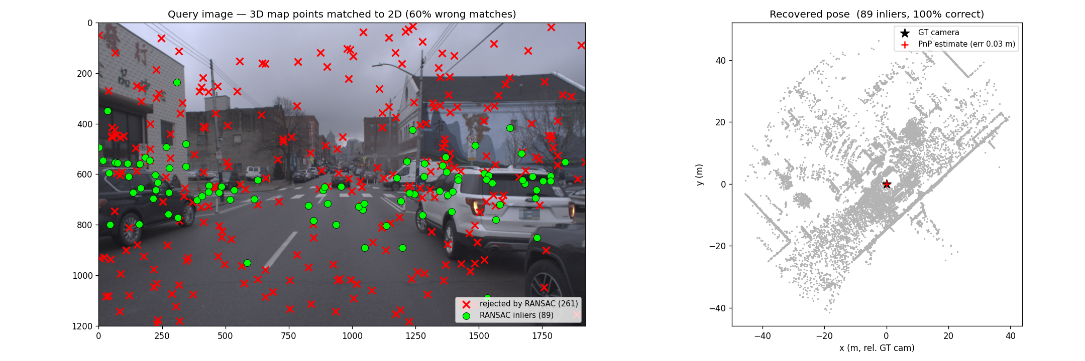
The key point: even though 60% of the data is garbage, PnP + RANSAC still recovers a pose accurate to cm level. It’s like asking a crowd for directions — a few people point the wrong way, each differently (random outliers), but everyone who actually knows points the same way; RANSAC just trusts that consensus. The correct matches are geometrically consistent (they all support one pose), while the wrong ones scatter harmlessly.

Road-map localization

The 4th direction: no a-priori feature map needed, only a free road map (OpenStreetMap) + relative motion from VO. A probabilistic filter tracks how likely the car is to be on each road segment: every segment starts equally likely, then each turn is a filtering step — a segment where that turn isn’t possible loses likelihood, while one where it fits gains it.

This is true localization (no initial position needed), converging after ~30–40 seconds even on a very large map. In exchange, it only knows the position along the road, not the full 6DoF pose.

Putting it together: VO – SLAM – Localization

• VO — estimates relative motion from images.
• SLAM — builds a map and localizes simultaneously; loop closure keeps the map consistent.
• Localization — uses that map (or a road map / GPS / HD map) to find the global pose.

A few principles:

• Indirect methods (feature-based) are fast and converge well but are less accurate; direct methods are slower but more accurate.
• Mapping can be done offline; but localization must be real-time because the ego pose has to be available immediately for downstream decisions.

Real-world deployment: sensor fusion

No sensor is perfect, so a real system integrates GNSS, IMU, LiDAR, camera, radar, and HD map — exploiting strengths and compensating weaknesses. Each source covers a specific gap:

• RTK-GNSS — position to ~1–3 cm (versus ~1 m with ordinary differential), but still drops out in tunnels / urban canyons.
• IMU/INS — high rate, fills the gaps between GNSS updates (5–10 Hz), but drifts without GNSS for too long.
• LiDAR — the decisive piece when GNSS is weak: matching the scanned point cloud against a pre-built map (e.g. with NDT).
• Camera — matching features / lane lines against an HD map (exactly the PnP example above).
• Wheel odometry — relative motion, independent of the external scene.

In short: GNSS-RTK + IMU gives a coarse, high-rate global frame; then LiDAR/camera map matching (feature-based + map-based) achieves cm accuracy and robustness in urban canyons and tunnels. Everything is fused by a state estimator.

Trends 2025–2026

• HD map + LiDAR (Waymo, Baidu Apollo, Mobileye): rely heavily on a pre-built HD map ⇒ very accurate, but the map production and maintenance pipeline is expensive, so HD maps only cover certain areas.
• Mapless, vision-centric: neural architectures processing camera + radar in real time, with no HD map or LiDAR ⇒ cheap, scalable but less accurate.
• Lite / crowdsourced maps and building HD maps online (Mobileye): a middle ground between the two extremes.