Visual Odometry Tutorial
Visual Odometry (VO), SLAM and Localization all revolve around estimating the motion of the ego agent. A self-driving car has to know how it is moving — as well as how the vehicles around it are moving.
VO estimates relative motion from images. It looks for the rigid-body transformation (R, t) — 6 degrees of freedom — between the scene at time t and time t+1. Unlike global localization, it chains poses incrementally and does not require a prior map. The word itself comes from the Greek hodos (route) + metron (measure).
In this post we implement the full Visual Odometry pipeline on the real-world Argoverse 1 dataset.
Notation used throughout
- ${}^{A}T_{B}$
- SE(3) transform mapping a point from frame $B$ into frame $A$ (equivalently, the pose of $B$ in $A$). In code:
A_SE3_B. - ${}^{A}R_{B}$, ${}^{A}t_{B}$
- the rotation and translation parts of ${}^{A}T_{B}$.
- $K$, $E$, $F$
- camera intrinsics, essential matrix, fundamental matrix.
Table of contents
- Data: a sequence from Argoverse
- Ground truth: the relative pose
- Moving to the camera coordinate frame
- VO: manually annotating correspondences
- Fitting epipolar geometry
- Recovering the relative motion
- Appendix: conventions & homogeneous coordinates
Data: a sequence from Argoverse
Argoverse is a large-scale public dataset for autonomous driving. Here we use only two images from the front-center camera. The data can be downloaded from Argoverse 1 (Training part 1 — each part contains several logs). The images are 1920×1200 px captured at 30 fps, and every log ships with the vehicle trajectory in a global frame (e.g. a city coordinate frame).
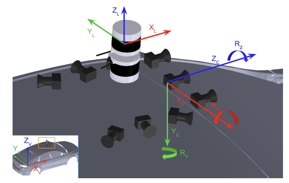
Goal: recover that trajectory from images alone, using 2D point correspondences. Argoverse uses the following coordinate convention: x forward (driving direction), y to the left of the vehicle, z up (against gravity).
Ground truth: the relative pose
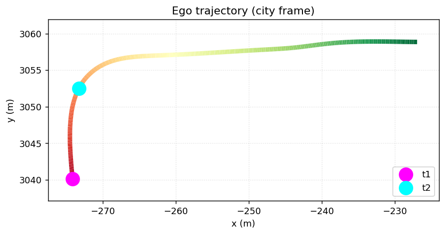
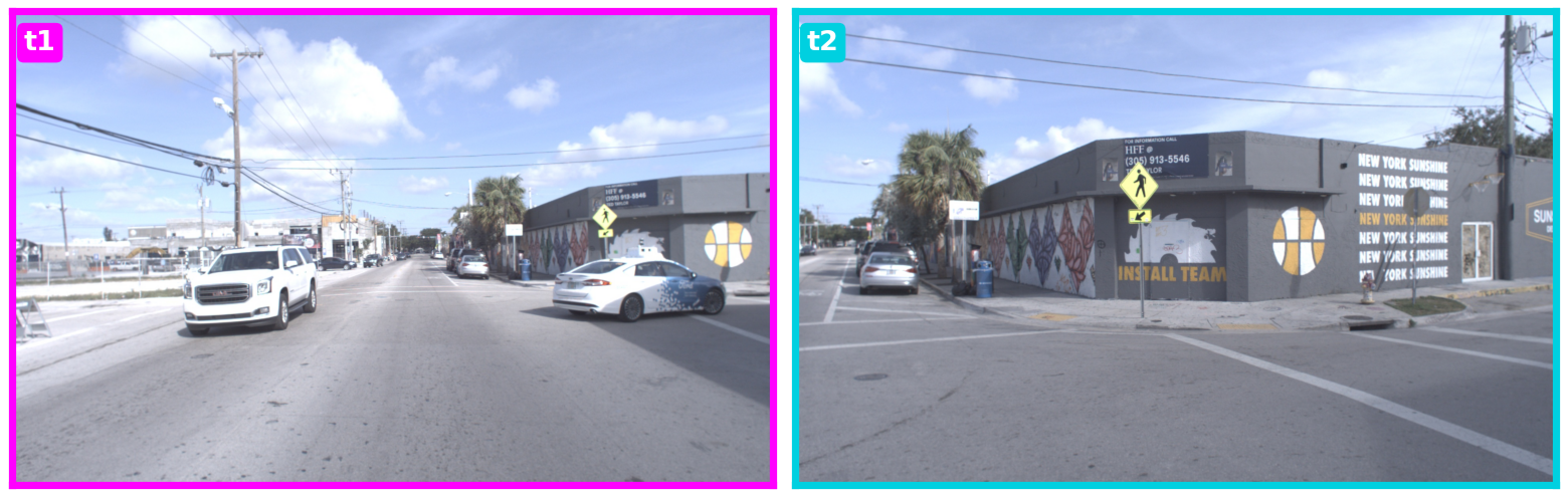
To measure accuracy we need the true relative pose between the two timestamps. We pick two instants on the trajectory and read off the vehicle pose at each (position is indexed by time).
ts1 = 315975640448534784  # nano-second timestamp
ts2 = 315975643412234000

log_id = '273c1883-673a-36bf-b124-88311b1a80be'
dataset_dir = '.../visual-odometry-tutorial/train1'

city_SE3_egot1 = get_city_SE3_egovehicle_at_sensor_t(ts1, dataset_dir, log_id)
city_SE3_egot2 = get_city_SE3_egovehicle_at_sensor_t(ts2, dataset_dir, log_id)

print(city_SE3_egot1.translation)   # ego position at t1 (city frame)
print(city_SE3_egot2.translation)   # ego position at t2
[-274.08 3040.12  -19.03]
[-273.25 3052.5   -19.1 ]
At each instant the SE(3) pose holds both a rotation and a translation:
- Translation — the position of the pose w.r.t. the global frame,
- Rotation — the orientation of the pose w.r.t. the global frame.
We want the relative pose between t1 and t2. We invert the first pose to go from global into the t1 frame, then compose:
# from t1 back to global
egot1_SE3_city = city_SE3_egot1.inverse()
# from t1 to t2
egot1_SE3_egot2 = egot1_SE3_city.compose(city_SE3_egot2)

from scipy.spatial.transform import Rotation
r = Rotation.from_matrix(egot1_SE3_egot2.rotation)
print(r.as_euler("zyx", degrees=True))        # yaw about z (egovehicle frame)
print(np.round(egot1_SE3_egot2.translation, 2))
[-32.47   0.59  -0.44]
[12.27 -1.88  0.  ]
In the egovehicle frame the relative rotation is a yaw of about −32.5° about the z-axis (a right turn), and the translation is about 12.3 m forward (along +x). The sign of the angle flips when we move to the camera frame in the next section.
Moving to the camera coordinate frame
A subtle but crucial point: the VO algorithm returns (R, t) between the two camera frames, not between the two vehicle frames. When we run the eight-point method on the 2D correspondences, what we recover is ${}^{c1}R_{c2}$ and ${}^{c1}t_{c2}$ — the motion of the camera between the two images.
So to check whether VO is correct, the ground truth (which lives in the ego frame) must be converted into the camera convention. We compose the ego pose with the fixed extrinsic transform ${}^{ego}T_{cam}$ read from the calibration file, so that both VO and ground truth are expressed in the same frame before we compare them.
# egovehicle_SE3_camera: read from vehicle_calibration_info.json
city_SE3_cam1 = city_SE3_egot1.compose(egovehicle_SE3_camera)
city_SE3_cam2 = city_SE3_egot2.compose(egovehicle_SE3_camera)
cam1_SE3_cam2 = city_SE3_cam1.inverse().compose(city_SE3_cam2)   # GROUND TRUTH (camera frame)

gt_rot = Rotation.from_matrix(cam1_SE3_cam2.rotation).as_euler("zyx", degrees=True)
print("Ground truth rotation:", np.round(gt_rot, 3))
print("Ground truth t       :", np.round(cam1_SE3_cam2.translation, 2))
Ground truth rotation: [-0.371 32.475 -0.422]
Ground truth t       : [ 2.64 -0.03 12.05]
As predicted, the yaw flips sign to +32.5° about the y-axis, and the translation is mostly along +z (the camera moves ~12 m forward). This is the (R, t) that VO will try to recover.
VO: manually annotating correspondences
To run VO we first need pairs of matching points across the two images. These correspondences can be estimated with classical methods (DoG + SIFT + RANSAC) or deep methods (SuperPoint + SuperGlue). For this tutorial we annotate them by hand using collect_ground_truth_corr.py, which uses matplotlib’s ginput() to let you click points on each image and save the correspondences to a pickle file.
export IMG_DIR=train1/273c1883-673a-36bf-b124-88311b1a80be/ring_front_center
python collect_ground_truth_corr.py \
  --img_fpath1 ${IMG_DIR}/ring_front_center_315975640448534784.jpg \
  --img_fpath2 ${IMG_DIR}/ring_front_center_315975643412234000.jpg \
  --experiment_name argoverse_2_E_1.pkl
Humans are not perfect, so each click carries some measurement error. We therefore annotate more correspondences than the strict minimum to average out the noise — at least 5 points for the essential matrix and 8 points for the fundamental matrix. In the pair below the car starts driving straight and then turns right; although there are several dynamic objects in the scene, plenty of static structure remains to match against.
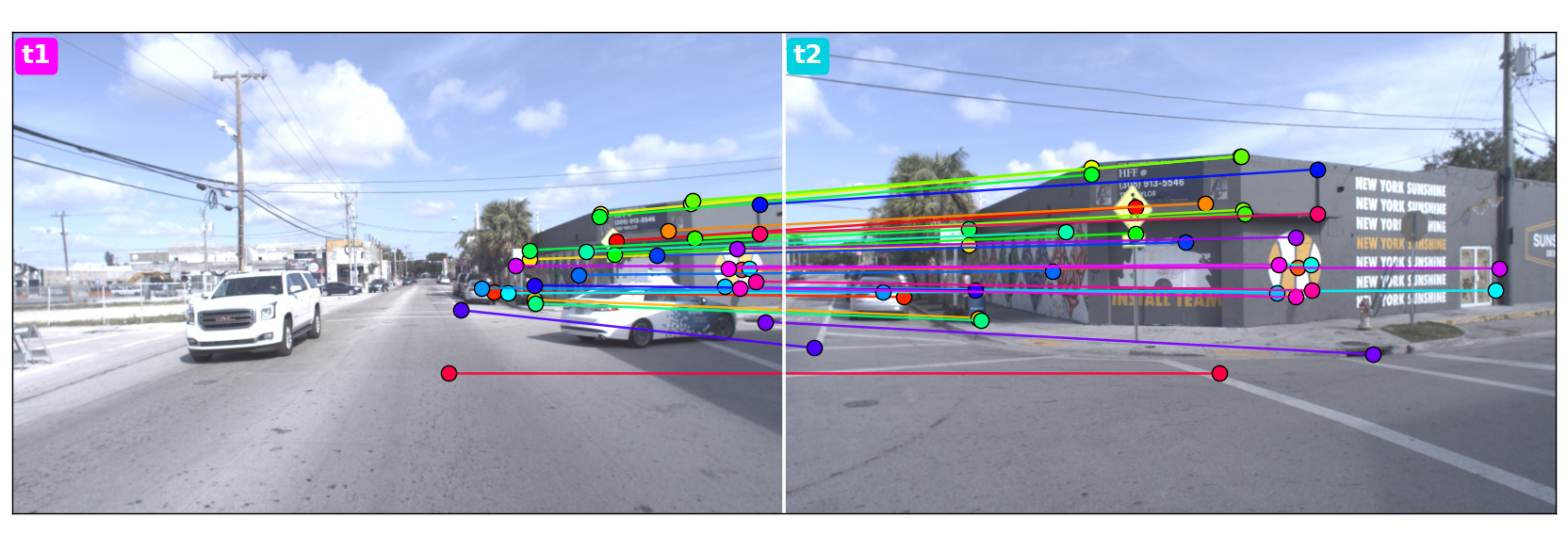
argoverse_2_E_1.pkl: each line links a point in image t1 (left) to the same physical point in image t2 (right), one colour per pair. Most points lie on static structure (buildings, poles, lane markings).Fitting epipolar geometry
We now fit the epipolar relationship. First we load the points we annotated:
import pickle
import numpy as np

pkl_fpath = '.../labeled_correspondences/argoverse_2_E_1.pkl'
with open(pkl_fpath, 'rb') as f:
    d = pickle.load(f)

X1, Y1 = np.array(d['x1']), np.array(d['y1'])  # points in image 1
X2, Y2 = np.array(d['x2']), np.array(d['y2'])  # points in image 2

# two Nx2 arrays of 2d-to-2d correspondences
img1_kpts = np.hstack([X1.reshape(-1,1), Y1.reshape(-1,1)]).astype(np.int32)
img2_kpts = np.hstack([X2.reshape(-1,1), Y2.reshape(-1,1)]).astype(np.int32)
There are two related matrices here. The fundamental matrix $F$ relates points in pixel coordinates and needs no knowledge of the camera. The essential matrix $E$ relates points in normalized (calibrated) coordinates and therefore requires the intrinsics $K$. They are related by $F = K^{-T} E K^{-1}$:
def get_fmat_from_emat(i2_E_i1, K1, K2):
    i2_F_i1 = np.linalg.inv(K2).T @ i2_E_i1 @ np.linalg.inv(K1)
    return i2_F_i1
Because the camera is the same at both poses, $K$ does not change. We estimate $E$ with OpenCV, using RANSAC to reject outliers:
import cv2
K = calib_dict['ring_front_center'].K[:3, :3]

cam2_E_cam1, inlier_mask = cv2.findEssentialMat(
    img1_kpts, img2_kpts, K, method=cv2.RANSAC, threshold=0.1)
print('Num inliers:', inlier_mask.sum())

cam2_F_cam1 = get_fmat_from_emat(cam2_E_cam1, K1=K, K2=K)
draw_epilines(img1_kpts, img2_kpts, img1, img2, cam2_F_cam1)
Num inliers: 9
(9 out of 33 hand-clicked points survive RANSAC — the rest are rejected as click noise.)
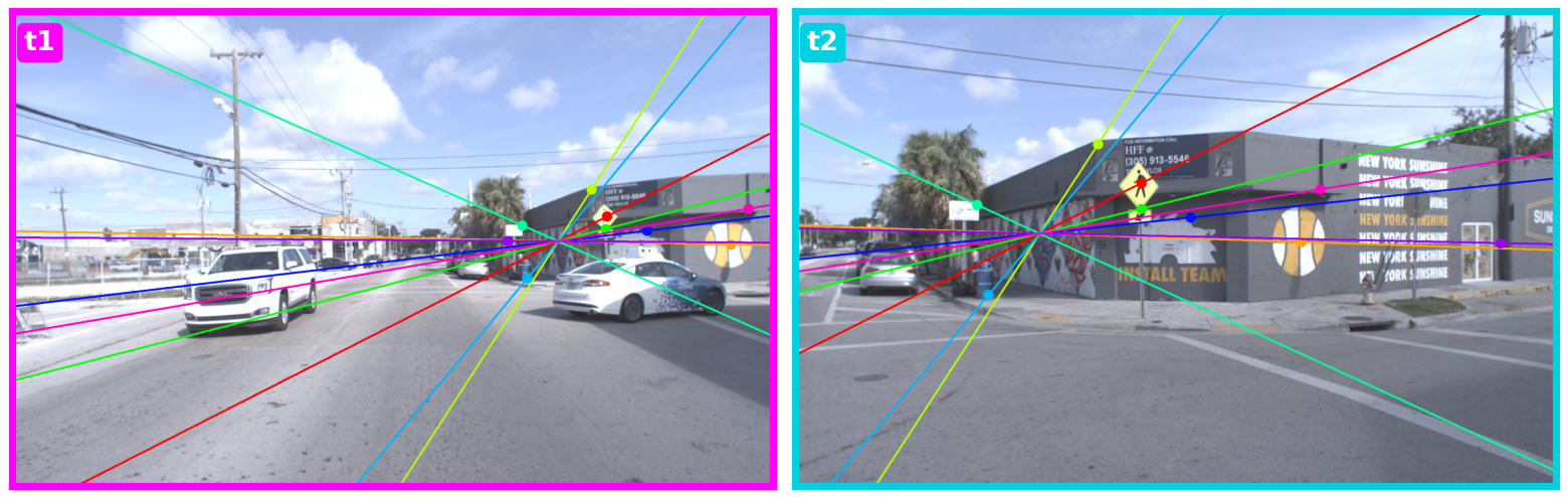
A good sanity check is to draw the epipolar lines. A point in one image corresponds to a 1D line in the other, and all epipolar lines converge at the epipole. Notice where the epipole lands in the left image: it is exactly where the front-center camera will be when the second image is captured. Using one color per correspondence, every point should lie on its epipolar line.
Recovering the relative motion
Finally we decompose the essential matrix into rotation and translation. OpenCV uses the 5-point algorithm under the hood:
_num_inlier, cam2_R_cam1, cam2_t_cam1, _ = cv2.recoverPose(
    cam2_E_cam1, img1_kpts, img2_kpts, K, mask=inlier_mask)

print(Rotation.from_matrix(cam2_R_cam1).as_euler('zyx', degrees=True))
print(np.round(cam2_t_cam1.squeeze(), 2))
[  0.4  -30.53   0.91]
[ 0.25  0.03 -0.97]
There is a catch. The recovered relative rotation is −30.5° rather than the expected +32°, and the translation points in −z instead of +z. The reason is that recoverPose returned the inverse transform (${}^{c2}R_{c1}$ instead of ${}^{c1}R_{c2}$). Inverting it and comparing directly against the ground truth:
# invert cam2_T_cam1 -> cam1_T_cam2, then compare to ground truth
cam1_SE3_cam2_est = SE3(cam2_R_cam1, cam2_t_cam1.squeeze()).inverse()
est_rot = Rotation.from_matrix(cam1_SE3_cam2_est.rotation).as_euler("zyx", degrees=True)
est_t_unit = cam1_SE3_cam2_est.translation / np.linalg.norm(cam1_SE3_cam2_est.translation)
gt_t_unit = cam1_SE3_cam2.translation / np.linalg.norm(cam1_SE3_cam2.translation)

print("Estimated rotation:", np.round(est_rot, 2))
print("Ground truth      :", np.round(gt_rot, 2))
print("Estimated t (unit):", np.round(est_t_unit, 3))
print("Ground truth t    :", np.round(gt_t_unit, 3))
Estimated rotation: [ 0.08 30.54 -0.83]
Ground truth      : [-0.37 32.47 -0.42]
Estimated t (unit): [ 0.274 -0.015  0.962]
Ground truth t    : [ 0.214 -0.002  0.977]
After inverting, the yaw is ≈ +30.5° (ground truth +32.5°) and the translation direction is off by only ~3.6° from ground truth — quite good for hand-clicked correspondences. VO recovers only the direction of the translation, not its scale (gauge ambiguity), so we compare unit vectors.
Appendix: conventions & homogeneous coordinates
1. Notation. ${}^{A}T_{B}$ (written A_SE3_B in code) is the transform that maps a point from frame $B$ into frame $A$ — equivalently, it is the pose of $B$ expressed in $A$.
2. Compose. Composing two SE(3) transforms is just multiplying their 4×4 matrices, so ${}^{A}T_{C} = {}^{A}T_{B} \cdot {}^{B}T_{C}$ (in code, A_SE3_C = A_SE3_B.compose(B_SE3_C)).
3. Why homogeneous coordinates? Translation is not a linear map, yet an SE(3) transform is a rotation followed by a translation. With plain 3-vectors you cannot fold rotation and translation into a single matrix multiply — you would have to apply $R$ and then add $t$ separately, which becomes painful when composing many steps.
Homogeneous coordinates fix this by adding one extra dimension: we lift a point $p$ to a 4-vector by appending a 1, and pack $R$ and $t$ into a single 4×4 matrix. A single multiply now does two jobs at once. It also handles projection: a camera projects a 3D point onto the 2D image by dividing by depth $Z$, and that division is not a linear operation — but the homogeneous convention absorbs it cleanly.