SLAM & Bundle Adjustment

In the Visual Odometry post, we recovered the relative motion (R, t) between two camera frames from corresponding points. Chaining many such pairs together reconstructs a whole trajectory. But every step carries a small error, and those errors accumulate over time (drift). SLAM tackles drift by no longer optimizing each step in isolation, but jointly optimizing all camera poses and all 3D points in a single problem.

SLAM = Simultaneous Localization And Mapping: estimating camera positions (localization) and a point map (mapping) at the same time. Just like in VO, once we have corresponding points across images (correspondences), we project each 3D point into every camera, measure the discrepancy against the observed position, then adjust both the camera and point positions so the total discrepancy is minimized. That is exactly Bundle Adjustment (BA) — a least-squares problem. Because the residual is nonlinear (projection, distance), we solve it iteratively with Gauss–Newton; and because the number of points is huge (tens of thousands in a self-driving setting), each iteration produces an enormous linear system — solved efficiently via the Schur complement.

In this post we build BA from scratch through 2 examples: a linear 1D problem to verify the formulas by hand, then a problem on a real Argoverse vehicle trajectory (the same dataset used in the VO post) — closing by building a real lidar map from the optimized trajectory.

Contents

• From Visual Odometry to SLAM
• The problem: nonlinear least squares
• Block structure of the Hessian & Schur complement
• Example 1 — linear 1D, checked against hand calculation
• Example 2 — a real Argoverse trajectory
• From trajectory to lidar map
• Appendix: Gauss–Newton, damping, gauge & observability

From Visual Odometry to SLAM

The VO post stopped here: from a pair of images and their correspondences, cv2.recoverPose gives us (R, t) between two cameras. That is a relative measurement, and it has two limitations:

1. Drift — chaining many (R, t) in a row accumulates error, so the trajectory gradually deviates.
2. Not all constraints used — a 3D point is usually seen from more than two cameras. Two-view VO wastes that information.

SLAM/BA solves both by setting up one optimization over everything: each 3D point $p_j$ seen from camera $c_i$ produces a residual (the difference between its observed position and its predicted position when the point is projected through the camera). The goal: simultaneously adjust every $c_i$ and $p_j$ so the sum of squared residuals is minimized.

The connection. The correspondences (point pairs) we labeled in the VO part are exactly the input to BA. VO provides a good initialization; BA refines it by using all observations at once.

The problem: nonlinear least squares

Let $x$ be all the unknowns (the positions of every camera — poses — and the positions of every point observed by the cameras — points). We minimize:

Since $r_k$ is nonlinear (projection, or computing the distance between two points — the l2 norm), we linearize around the current estimate: $r(x+\delta) \approx r(x) + J\delta$, then solve for the update step $\delta$ via the normal equations:

$H\delta = -g$,   with $H = J^\top J$, $g = J^\top r$

This is Gauss–Newton: $H = J^\top J$ is an approximate Hessian (dropping the second-order derivative of $r$), good enough when residuals are small. Repeat until convergence.

In other words: linearize the objective at the starting point, solve the update step by setting the derivative to zero, move the estimate to the optimum within that linearized region, then linearize again around the new estimate and solve again — repeating until the estimate barely changes.

If we build the full $H$ directly and solve, the cost is $O(n^3)$ with $n$ = total number of unknowns — infeasible with thousands of points. This is where the block structure comes in.

Block structure of the Hessian & Schur complement

Splitting the unknowns into two groups — cameras (c) and points (p) — gives $H$ an arrowhead structure:

• $U$ — the camera–camera block (small, on the order of the number of cameras).
• $V$ — the point–point block, block-diagonal: each point is independent of the others ⇒ extremely cheap to invert.
• $W$ — the camera–point coupling block (sparse: nonzero only when camera $i$ sees point $j$).

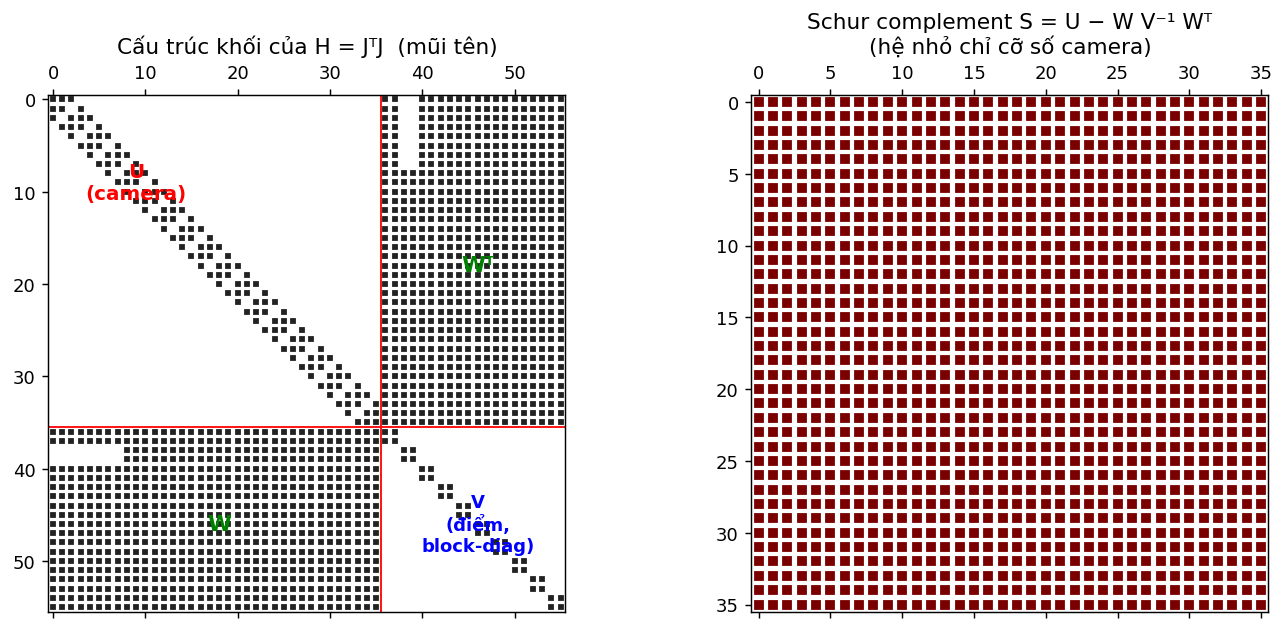
The Schur complement exploits exactly this structure, splitting $H\delta = -g$ into 4 steps (this is what COLMAP, g2o, and Ceres do internally):

1. $V^{-1}$  (cheap because block-diagonal)
2. $S = U - W V^{-1} W^\top$  (Schur complement)
3. solve for $\delta_c$: $S\,\delta_c = -(g_c - W V^{-1} g_p)$
4. back-substitute: $\delta_p = -V^{-1}(g_p + W^\top \delta_c)$

The key point: we only need to solve the system $S$ of size the number of cameras (a few dozen) instead of the whole $H$ of size cameras-plus-points (thousands). Everything else in this post is just assembling $U, V, W, g_c, g_p$ from the Jacobian and then calling this function:

import numpy as np

def solve_schur(U, W, V, gc, gp, lam=0.0):
    U = U + lam*np.eye(U.shape[0])      # Levenberg–Marquardt damping (see appendix)
    V = V + lam*np.eye(V.shape[0])
    Vinv = np.linalg.inv(V)             # 1) invert V (block-diagonal -> cheap)
    S  = U - W @ Vinv @ W.T             # 2) Schur complement
    dc = np.linalg.solve(S, -(gc - W @ Vinv @ gp))   # 3) solve for delta_c
    dp = -Vinv @ (gp + W.T @ dc)        # 4) back-substitute for delta_p
    return dc, dp, S

Example 1 — linear 1D, checked against hand calculation

We start with the simplest possible model to verify the formulas: everything lies on a single axis.

• 2 cameras $c_0, c_1$; 3 points $p_0, p_1, p_2$.
• Each observation measures a “distance” $m = p_j - c_i$ ⇒ residual $r = (p_j - c_i) - m$, so $\partial r/\partial c_i = -1$, $\partial r/\partial p_j = +1$.
• Add 1 prior pinning $c_0$ to fix the gauge (see appendix).

Because the model is linear, Gauss–Newton converges in exactly 1 step:

cams_gt = np.array([1.0, 2.0])
pts_gt  = np.array([3.0, 7.0, 10.0])
obs = [(0,0),(0,1),(1,1),(1,2)]              # cam0 sees p0,p1 ; cam1 sees p1,p2
m = np.array([pts_gt[j]-cams_gt[i] for i,j in obs])

c = np.array([0.0, 0.0]); P = np.array([0.0, 0.0, 0.0])    # init away from the solution
nc, npt = 2, 3
U=np.zeros((nc,nc)); V=np.zeros((npt,npt)); W=np.zeros((nc,npt))
gc=np.zeros(nc); gp=np.zeros(npt)
for (i,j),mij in zip(obs,m):
    r=(P[j]-c[i])-mij; Jc,Jp=-1.0,1.0
    U[i,i]+=Jc*Jc; V[j,j]+=Jp*Jp; W[i,j]+=Jc*Jp     # accumulate J^T J into the right block
    gc[i]+=Jc*r;   gp[j]+=Jp*r
r=(c[0]-cams_gt[0]); U[0,0]+=1; gc[0]+=r            # prior pinning cam0

dc,dp,S = solve_schur(U,W,V,gc,gp)
# S       -> [[ 1.5 -0.5]   <-- matches the hand calculation exactly
#             [-0.5  0.5]]
# c+dc    -> [1. 2.]   (= cams_gt)
# P+dp    -> [ 3.  7. 10.]   (= pts_gt)

# Cross-check: Schur gives the EXACT same result as solving the full H directly
H=np.block([[U,W],[W.T,V]]); g=np.concatenate([gc,gp])
full=np.linalg.solve(H,-g)
# np.allclose(np.concatenate([dc,dp]), full) -> True

Two things to take away: (1) $S$ comes out exactly $\begin{bmatrix} 1.5 & -0.5 \ -0.5 & 0.5 \end{bmatrix}$ as in the hand calculation; (2) solving via Schur equals solving the full $H$ directly — Schur is just a faster way to solve, it does not change the solution.

Example 2 — a real Argoverse trajectory

Now running on real data. We read the pose files city_SE3_egovehicle_*.json of an Argoverse 1 log directly — the same dataset used in the VO post — and take the vehicle position $(x, y)$ as the ground-truth trajectory.

Unlike Example 1 (linear, solved in one shot), the measurement here is a Euclidean distance, so the residual is nonlinear ⇒ $J, r$ must be recomputed every Gauss–Newton iteration. The way they are accumulated into $U, V, W$ is identical — and solve_schur still doesn’t change by a line.

import json, glob, os
LOG = "data/.../train1/e17eed4f-3ffd-3532-ab89-41a3f24cf226"
pf = sorted(glob.glob(os.path.join(LOG,"poses","city_SE3_egovehicle_*.json")),
            key=lambda p:int(p.split("_")[-1].split(".")[0]))
xy = np.array([json.load(open(p))["translation"][:2] for p in pf])
gt = xy[::40][:18]; gt = gt - gt[0]          # every 40 frames, 18 poses, recentered to origin
N = len(gt)
# N = 18 ; span ~ 18.6 x 17.2 m  (a stretch where the car is turning)

On that trajectory we build a 2D SLAM problem — this is where all the pieces come together:

• Camera = the vehicle position at each timestamp (the 2D unknown to find) — analogous to pose in VO.
• Landmark = a few marker points scattered around the road (simulating lamp posts / signs that lidar would pick up).
• Range observation: each pose measures the distance to landmarks within a 40 m radius (noisy) — playing the role of correspondences in VO.
• Odometry: the relative displacement between 2 adjacent poses (noisy) — exactly the $(R, t)$ that VO produces; it creates a camera–camera constraint (the off-diagonal band in block $U$ above).
• Prior: fix pose0 (gauge) + a loose landmark prior to resolve range-only ambiguity.

We initialize with dead-reckoning (accumulating noisy odometry) → the trajectory gradually drifts; then BA uses ranges to landmarks to pull it back close to the ground truth. This is exactly why SLAM is needed: odometry alone drifts, and the landmark map corrects it.

rng = np.random.default_rng(0)
mn, mx = gt.min(0)-15, gt.max(0)+15
L_gt = rng.uniform(mn, mx, size=(10,2)); M = len(L_gt)
obs = [(i,l, np.hypot(*(L_gt[l]-gt[i])) + rng.normal(0,0.15))    # noisy range
       for i in range(N) for l in range(M) if np.hypot(*(L_gt[l]-gt[i])) < 40]
odo = [(i, gt[i+1]-gt[i] + rng.normal(0,0.7,2)) for i in range(N-1)]   # drifting odometry
# n range obs = 176 ; n odo = 17

x = np.zeros((N,2))                              # init = dead-reckoning
for i,o in odo: x[i+1] = x[i] + o
x_dr = x.copy()
L_prior = L_gt + rng.normal(0,3,size=L_gt.shape); Lh = L_prior.copy()
wp, wl = 10.0, 0.6                               # prior weights for pose0 / landmark
ci = lambda i: slice(2*i,2*i+2); li = lambda l: slice(2*l,2*l+2)

for it in range(30):
    U=np.zeros((2*N,2*N)); V=np.zeros((2*M,2*M)); W=np.zeros((2*N,2*M))
    gc=np.zeros(2*N); gp=np.zeros(2*M); cost=0.0
    for i,l,z in obs:                            # --- range residual (camera <-> point) ---
        dvec=Lh[l]-x[i]; d=np.hypot(*dvec)+1e-9; r=d-z; cost+=r*r
        Jx=-dvec/d; JL=dvec/d
        U[ci(i),ci(i)]+=np.outer(Jx,Jx); gc[ci(i)]+=Jx*r
        V[li(l),li(l)]+=np.outer(JL,JL); gp[li(l)]+=JL*r; W[ci(i),li(l)]+=np.outer(Jx,JL)
    for i,o in odo:                              # --- odometry residual (camera <-> camera) ---
        r=(x[i+1]-x[i])-o; cost+=r@r; I=np.eye(2)
        U[ci(i),ci(i)]+=I; U[ci(i+1),ci(i+1)]+=I
        U[ci(i),ci(i+1)]-=I; U[ci(i+1),ci(i)]-=I
        gc[ci(i)]+=-r; gc[ci(i+1)]+=r
    r=wp*x[0]; U[ci(0),ci(0)]+=wp*wp*np.eye(2); gc[ci(0)]+=wp*r; cost+=r@r   # gauge
    for l in range(M):                           # loose landmark prior
        rl=wl*(Lh[l]-L_prior[l]); V[li(l),li(l)]+=wl*wl*np.eye(2); gp[li(l)]+=wl*rl; cost+=rl@rl
    dc,dp,_=solve_schur(U,W,V,gc,gp,lam=1e-2)    # <-- still the same function as Example 1
    x=x+dc.reshape(-1,2); Lh=Lh+dp.reshape(-1,2)
# cost: 4668 -> 119 (floor = measurement noise) after ~3 iterations
# Trajectory error (RMSE vs ground-truth):
#   dead-reckoning = 3.709 m   ->   after BA = 1.478 m   (2.5x reduction)

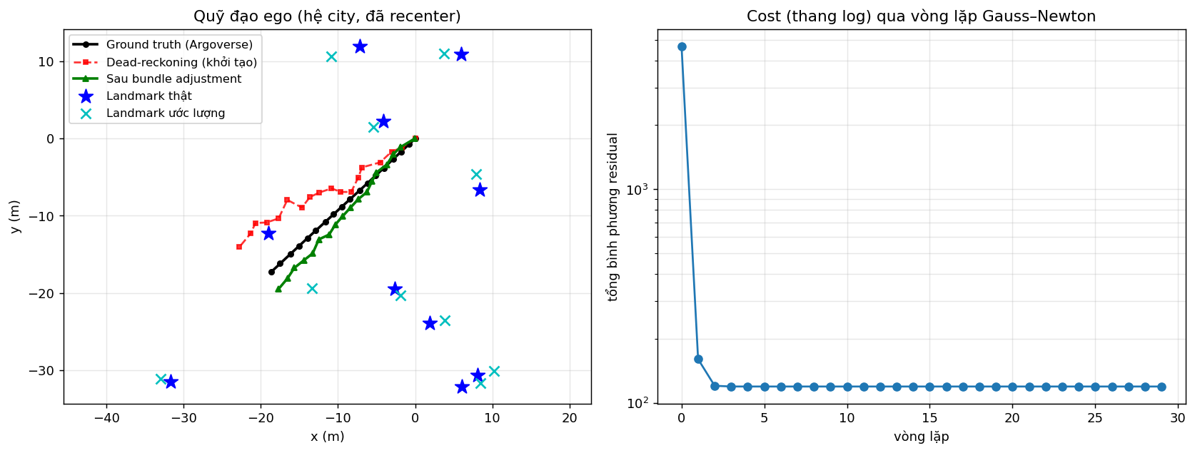
Worth noting: the solve_schur function from Example 1 does not change by a single line — from the 1D hand-checked problem to SLAM on a real vehicle, only the way $U, V, W$ are assembled differs. That is precisely the power of splitting the problem along its block structure.

From trajectory to lidar map

So far we have only done half the “L” (localization — the trajectory). The other half, “M” (mapping), is almost free: once we have a good trajectory, we simply take the lidar point cloud at each pose (in the vehicle frame) and place it into a common frame using that pose — overlapping sweeps reinforce each other into a map.

One small difference: lidar also needs the vehicle’s orientation, so here the pose is SE(2) $(x, y, \theta)$ — adding the angle $\theta$ compared to the range-only problem above. The Gauss–Newton + Schur machinery is unchanged; the residual simply gains an angular term (full code in the notebook). The map-aggregation function is just a rotate by $\theta$ then translate:

def aggregate(poses, sweeps):       # poses: (N,3) = (x, y, theta) ; sweeps[i]: lidar points, vehicle frame
    pts = []
    for (x, y, th), p_ego in zip(poses, sweeps):
        c, s = np.cos(th), np.sin(th)
        X = c*p_ego[:,0] - s*p_ego[:,1] + x        # rotate by yaw + translate -> map frame
        Y = s*p_ego[:,0] + c*p_ego[:,1] + y
        pts.append(np.c_[X, Y])
    return np.concatenate(pts)
# trajectory RMSE:  dead-reckoning = 2.85 m   ->   after BA = 0.11 m   (78 sweeps, ~1.7M points)

The same set of lidar sweeps, placed by three different trajectories:

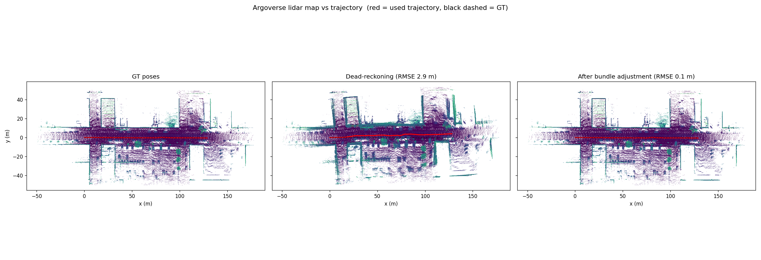
This is the most visual reason why SLAM matters: good poses ⇒ a sharp map. Drift offsets the sweeps so the same wall gets drawn as several layers; BA corrects the poses so those layers overlap cleanly. The next step toward a complete SLAM system is loop closure (detecting a revisit) — adding camera–camera constraints between far-apart poses, which still fit inside block $U$ and the same solve_schur.

Appendix: Gauss–Newton, damping, gauge & observability

1. Gauss–Newton vs Levenberg–Marquardt. We approximate the Hessian by $J^\top J$ (dropping the second-order term). When far from the solution, or when $S$ is near-singular, the Gauss–Newton step can “jump” badly. The lam parameter in solve_schur adds a small $\lambda I$ to the diagonal — that is Levenberg–Marquardt damping: large $\lambda$ → small, cautious step (like gradient descent); small $\lambda$ → fast Gauss–Newton step.

2. Gauge freedom. If we shift the entire scene (all cameras and points) by the same amount, every relative distance/observation is unchanged ⇒ the cost is unchanged ⇒ the problem has infinitely many solutions. This is gauge freedom. We remove it with a prior fixing one anchor (pose0 in Example 2). This phenomenon is a relative of the scale ambiguity in the VO post: there, VO only recovers the direction of the translation, not its scale, so we compare unit vectors.

3. Observability (range-only ambiguity). With distance-only measurements, a landmark and its mirror image across the path give the same set of distances ⇒ cost = 0 for several different scenes. Drop all priors and BA may converge to a scene that is “right in the numbers but wrong in shape”. Loose priors (w_prior, wl) and increasing observation coverage make the problem well-posed. This is a genuine observability issue of SLAM, not a code bug.

4. Things to try. Reduce obs (a more weakly-constrained problem), increase the range/odo noise, raise lam (more cautious steps), or drop the priors to see the range-only ambiguity. The next step toward real BA in COLMAP/VO: replace the distance residual with reprojection error (the pixel error when projecting a 3D point through the camera) — exactly the model the Visual Odometry post laid the groundwork for.